 This example
will be used throughout to illustrate a complete solution. All the data has
been made up in these examples.
by Patrick Warren
The aim of this article is to present a new method for distributing misclosure errors encountered in surveying complicated network caves. The hope is that this will form the basis of an efficient computer algorithm which will not use much memory or take much time.
Two examples are treated in detail: the first demonstrates the general method and the second demonstrates powerful ways of distributing errors from large loops across smaller loops, without the use of a computer.
The method has a firm basis in the theory of the least squares solution to such problems. This solution I worked out independently a couple of years ago and made the basis of a computer program which appeared in a CPC Journal [1]. The program was very slow and I was convinced there was a better solution. After spending a couple of weeks playing with the basic equations, in Dec 1986 I rearranged them into the more elegant form presented below, which is much more efficient than the original program. It remains yet to convert these new methods into a computer algorithm, but that should not be too difficult (I have already talked to a willing computer programmer).
I choose not to present the full development from the conception of the least squares solution to the form presented here for several reasons. Firstly there is an awful lot of algebraic manipulation involved which would have taken up most of this journal. Secondly not many people would be interested in, or want to follow all the gory details of such a derivation. Thirdly I hope to collect all my results into one paper (as yet unwritten) and get it published.
I have talked to several people about the method of least squares, and it appears that very little has been published in this country about it, although it is used in America. I would consider the method to be the optimum solution to the problem of misclosures: it solves the problem in one go and is not an iterative solution; it works no matter how complicated the network becomes; finally if the data put in (ie. the northing, easting and height change for each leg) is normally distributed with the same standard deviation for each bit (this is usually true), I believe the least squares solution gives the most probable answers for the station positions given the data in the problem (ie. it is the maximum likelihood estimate in statistical language). I have not fully proved this last point to my satisfaction, but it seems reasonable. Indeed the whole problem of the statistical treatment of survey data seems untouched by human hand as yet, and appears to be very complicated especially in the presence of loops or networks.
I hope the reader manages to wade through the rest of this article, and at the end he or she at least appreciates the problem of misclosure errors has largely been solved (even if he or she does not want to use the methods anyway!)
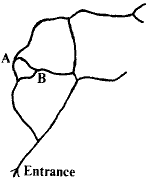
Suppose we had surveyed a cave system whose centre line is that illustrated below:
 This example
will be used throughout to illustrate a complete solution. All the data has
been made up in these examples.
The data is in the form of length, clino and bearings for a large number of survey legs taken between a large number of survey stations. The aim of the article is to explain how to convert these data to the coordinates of the survey stations and so to draw out the survey.
First we must make clear what we mean by certain words and definitions. Probably every surveyor knows what is meant by survey stations and survey legs - stations and legs for short. A length of passage where there is no branching off is called a section (at least by me) and those survey Stations which lie at branching points are called vertex stations or vertices for short.
Thus in the diagram above, A and B are vertices, whilst the centre line
directly connecting the two (A->B) is a section.
In more detail, the centre line from A to B might be:
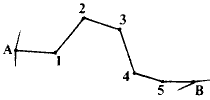 The entries
in the surveyors notebook are in the following form:
From To   Length Clino Bearing

1    2    5.02 m  +01   010

etc...
We have to convert these to displacements in height, easting and northing.
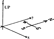
If we use the standard coordinate system below, we can write
![]() x,
x,
![]() y,
y,
![]() z for the changes
in easting, northing and height respectively and we can calculate these for
any leg.
z for the changes
in easting, northing and height respectively and we can calculate these for
any leg.
Writing '![]() '
for the inclination,
'
'
for the inclination,
'![]() ' for the bearing
and L for the length we get:
' for the bearing
and L for the length we get:
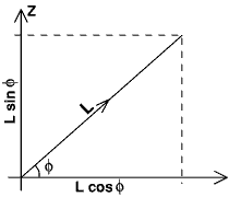
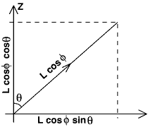
![]() x = L cos(
x = L cos(![]() ) sin(
) sin(![]() ) = easting change
) = easting change
![]() y = L cos(
y = L cos(![]() ) cos(
) cos(![]() ) = northing change
) = northing change
![]() z = L sin(
z = L sin(![]() ) = height change
) = height change
Note that the triple
(![]() x,
x,
![]() y,
y,
![]() z) goes
from one station to another which we indicate by putting an
arrow on the line representing the leg:
z) goes
from one station to another which we indicate by putting an
arrow on the line representing the leg:

Thus we might have the following data for part of the section from A to B
above

| From | To | L/m | ' |
' |
---> | |||
|---|---|---|---|---|---|---|---|---|
| 1 | 2 | 5.02 | 010 | +01 | 0.87 | 4.94 | 0.09 | |
| 3 | 2 | 8.70 | 297 | +02 | * | -7.75 | 3.95 | 0.30 |
| 3 | 4 | 2.98 | 135 | -05 | 2.10 | -2.10 | -0.26 |
There are similar entries for every leg in the whole survey, section by section.
This section was surveyed by the leapfrog method, and we must convert all
the readings in a section to be in the same direction. This can be
accomplished by changing the sign of the
![]() x,
x,
![]() y,
y,
![]() z.
z.
ie: If ![]() has
has
![]() x,
x,
![]() y,
y,
![]() z.
z.
then ![]() has
-
has
-![]() x,
-
x,
-![]() y,
-
y,
-![]() z.
z.
So converting the entry marked * to be a forward reading we get
| From | To | |||
|---|---|---|---|---|
| 2 | 3 | 7.75 | -3.95 | -0.30 |
We treat the other backward entries in a similar manner.
We can now work out the total displacements in easting, northing and
height as we go from station A to station B. We denote these by
![]() xAB,
xAB,
![]() yAB,
yAB,
![]() zAB.
We get these by adding up all the
zAB.
We get these by adding up all the
![]() x,
x,
![]() y,
y,
![]() z, for the
individual legs. Thus we might have for the section A to B (only doing the x
coordinates) the following:
z, for the
individual legs. Thus we might have for the section A to B (only doing the x
coordinates) the following:

| From | To | |||
|---|---|---|---|---|
| A | 1 | 5.35 | -- | -- |
| 1 | 2 | 0.87 | 4.94 | 0.09 |
| 2 | 3 | 7.75 | -3.95 | -0.30 |
| 3 | 4 | 2.10 | -2.10 | -0.26 |
| 4 | 5 | 3.21 | -- | -- |
| 5 | B | 2.07 | -- | -- |
| ----- 21.35 |
For each section we also have to take account of the number of legs which we denote by n. For the section above, nAB = 6.
The section A->B we show diagrammatically as

![]() x = 21.35m,
n = 6
x = 21.35m,
n = 6
(![]() y = ----,
y = ----,
![]() z = ----)
z = ----)
From now on we concentrate on the x coordinates of the stations since the procedure for calculating the y and z coordinates is identical. We will remind the reader of this generalisation at various points.
For brevity we drop the 'x' in some of the symbols thus:
![]() xAB
->
xAB
->
![]() AB
AB
ExAB -> EAB
exAB -> eAB
The last two will be defined in the next section. Now we must introduce some more ideas.
i) All the survey stations will have absolute positions in some coordinate system whose origin, however, is still arbitrary. The aim is of course to calculate these positions. We denote these by x,y,z. Thus A has xA, yA, zA, B has xB, yB, zB and so on for each station in the survey. The general set of these is denoted by xA, xB, ... As we said above, we are implicitly including the y and z coordinates of all the stations in all this. As already stated, the aim is to calculate the set xA, xB, ...
Note that any calculation will lead to values for the coordinates of the survey Stations, but only to within an arbitrary constant. This is because the origin of the coordinate System is arbitrary. To obtain actual answers for the coordinates of the survey Stations, we must include an additional fact or constraint, namely the position of some basis Station in the coordinate system. Usually this will be the entrance fixed at x=0, y=0, z=0 but it need not be.
ii) Due to misclosure errors, the displacement xB -
xA may not be exactly equal to the measured displacement
![]() AB.
The difference is called the total error for the section and is given the
symbol EAB.
AB.
The difference is called the total error for the section and is given the
symbol EAB.
| EAB = xB - xA -
|
[More properly EcAB = xB -
xA -
|
Also defined is the fractional error for a section, or error per leg which is given the symbol e.
eAB = EAB / nAB
Note that we have to solve the full problem to determine what xA and xB are before we can calculate E and e for a Section.
[With all three coordinates there are three E's and three e's for each section, ExAB, EyAB, EzAB; exAB, eyAB, ezAB; defined like the above.]
When we have solved the problem and determined EAB and eAB, we can distribute this error back along the section to determine the actual coordinates of the intermediate stations.
Thus for our example, for Section A->B, the relevant formulæ are:
 x1 = xA +
![]() xA1
+ eAB,
xA1
+ eAB,
x2 = xA +
![]() xA1 +
xA1 +
![]() x12
+ 2eAB,
x12
+ 2eAB,
etc...
Later on we shall solve the problem of the network, and obtain values for xA and xB. But here we pinch these answers to illustrate the distribution of errors back along a section.
We get xA = -17.97m, xB = 3.64m, and we already know
![]() AB =
21.35m, nAB = 6 from above. Thus
AB =
21.35m, nAB = 6 from above. Thus
EAB = 3.64 - (-17.97) - 21.35 = 0.26m
eAB = 0.26 / 6 = 0.0437m
We can now calculate the positions of Stations 1...5
| From | To | Positions | |
|---|---|---|---|
| xA = -17.97m | |||
| A | 1 | 5.35 | x1 = -12.58m |
| 1 | 2 | 0.87 | x2 = -11.66m |
| 2 | 3 | 7.75 | x3 = -3.87m |
| 3 | 4 | 2.10 | x4 = -1.73m |
| 4 | 5 | 3.21 | x5 = 1.53m |
| 5 | B | 2.07 | xB = 3.64m |
for example:
x3 = x2 +
![]() x23 + e
x23 + e
= -11.6635 + 7.75 - 0.0437
= -3.8698
= -3.87 [To 2 dec. places]
The calculation was done to 4 dec. plac. but the results were written to 2 dec. plac.
How did we obtain the values of xA and xB in the first place?
The least squares method leads, after much algebraic manipulation, to the following solution.
The xA, xB, ... are treated as unknown variables which are to be solved for simultaneously. Then for each section (for example A to B) the fractional error is eAB.
|
eAB = [ xB - xA -
|
- a function of the xA, xB, ... |
At each vertex station write the equation,
Sections entering |
- | Sections leaving | = 0 |
or Algebraic sum of e's of sections connected to this vertex = 0
This gives us an equation involving the xA, xB, ...'s at each vertex (but often only a few of them at a time).
There are N vertices giving N equations, and there are N unknowns xA, xB, ... These equations, together with the condition that the position of one of the xA, xB, ...'s is specified (as mentioned above), can be solved simultaneously and the solution is the least squares solution to the problem (this is not an obvious statement - the proof is long and convoluted).
The best way to illustrate this is to plunge into a meaty example
Suppose we had the survey shown at the start:
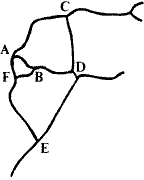 We can ignore those sections which do not form part of a loop (justified
below) and we get:
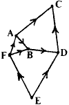 We have labelled the important vertex stations A...F.
Suppose we had the following data for the sections - which would be worked out for each section from the individual legs as we did in the example A->B. [The first two columns are the data, the last three are worked out from the solution and are there for comparison.]
| From | To | x/m | n | xto - xfrom/m | E/m | e/m |
|---|---|---|---|---|---|---|
| A | B | 21.35 | 6 | 21.61 | 0.26 | 0.0437 |
| F | A | 9.77 | 7 | 9.85 | 0.08 | 0.0118 |
| F | B | 31.98 | 7 | 31.46 | -0.51 | -0.0736 |
| B | D | 31.77 | 7 | 31.56 | -0.21 | -0.0299 |
| E | F | -27.02 | 13 | -27.82 | -0.80 | -0.0618 |
| E | D | 34.09 | 18 | 35.20 | 1.11 | 0.0618 |
| A | C | 58.21 | 16 | 57.70 | -0.51 | -0.0319 |
| D | C | 4.11 | 13 | 4.53 | 0.42 | 0.0319 |
| These columns are the data. | These columns are worked out from the answers. | |||||
For each vertex we are told to write
![]() e = 0.
e = 0.
For A : (xA - xF - 9.77)/7 -
(xB - xA - 21.35)/6 -
(xC - xA - 58.21)/16 = 0
For B : (xB - xF - 31.98)/7 +
(xB - xA - 21.35)/6 -
(xD - xB - 31.77)/7 = 0
For C : (xC - xA - 58.21)/l6 -
(xD - xC - 4.11)/13 = 0
For D : (xD - xB -31.77)/7 +
(xD - xE - 34.09)/18 -
(xC - xD - 4.11)/13 = 0
For E : - (xF - xE + 27.02)/13 -
(xD - xE -34.09)/18 = 0
For F : (xF - xE + 27.02)/13 -
(xA - xF - 9.77)/7 -
(xB - xF - 31.98)/7 = 0
Taking these together with the basis station xE = 0.00m gives the complete solution (using a computer - although this example is just about manageable by hand).
| xA = -17.97m | xD = 35.20m |
| xB = 3.64m | xE = 0.00m |
| xC = 39.73m | xF = -27.82m |
These answers are put back into the last three columns of the table above. The E and e for each section is worked out, allowing us to distribute the errors back along each section exactly as was done for the A->B case.
i) Hopefully the method described above will form the basis of a computer algorithm for the calculation of survey coordinates since the calculation for even a simple network is very lengthy and error-prone by hand. Even using the special techniques described in the next section (especially in parts 3 and 4), only a few networks are amenable to treatment by hand.
ii) We can calculate the y and z coordinates of the stations in an exactly
similar manner to the way we calculated the x coordinates. The coefficients
of the yA .. yF or zA .. zF
remain the same, it is only the constant terms which change as the
{![]() x} is replaced by
{
x} is replaced by
{![]() y} or
{
y} or
{![]() z). Effectively
this means the equations need only be solved once, not three times.
Furthermore the equations seem to be naturally well conditioned, so
implementation on a computer is made easier.
z). Effectively
this means the equations need only be solved once, not three times.
Furthermore the equations seem to be naturally well conditioned, so
implementation on a computer is made easier.
iii) It is recommended to keep numbers to four or more places of decimals during the intermediate stages of the calculation. This is to avoid rounding errors which in the example above would give rise to greater errors than were present in the actual data for some of the sections. Thus the e are given to four places of decimals, even though the legs aren't measured to this accuracy, so that the positions of the intermediate stations can be calculated correctly. At the end of the calculations, the positions of the stations can be (and should be) given to two places of decimals, with no uncertainty in the last place arising from rounding errors made during the calculations.
We now derive some more advanced results which tie in with what we would expect from common sense.
1) This is the proof of a step taken in our previous example, namely that we can ignore those sections which do not form part of a loop.
We look at the situation where we have a section attached at one end only,
 which can be
represented as
| At C we write | (1) | |
| At D we write | [xD - xC -
| (2) |
![]() 'e means the
sum over the other sections attached to C.
'e means the
sum over the other sections attached to C.
From (2) we get xD = xC +
![]() CD
CD
Hence ECD and eCD are both zero, there are no errors to distribute, and we get the positions of the intermediate stations by just adding up the individual displacements needed to reach them. This of course is what we would expect.
Put (2) into (1) and get
![]()
![]() 'e = 0
which just represents ...
'e = 0
which just represents ...
[ie: it is what we would write down if we just had the above.]
This shows we can ignore the sections which are not part of a loop, and then add them back in later on.
This proof generalises easily. For example,
 goes to
 goes to
 goes to
 etc...
2) What happens if we have a loop for example?

What do we write for the equation at P?
It is not just
![]() 'e +
[xP - xP -
'e +
[xP - xP -
![]() 1]
/ n1 = 0
1]
/ n1 = 0
We must include the fact that the same section leaves as well as enters station P and write
![]() 'e +
[xP - xP -
'e +
[xP - xP -
![]() 1]
/ n1 -
[xP - xP -
1]
/ n1 -
[xP - xP -
![]() 1]
/ n1 = 0
1]
/ n1 = 0
or ![]() 'e = 0
'e = 0
So we can ignore the loop just as we ignored the odd section attached at one end as in part 1).
What happened to the information in the loop (there is no counterpart to equation (2) here)?
The answer is that we don't need it since we atready know E1 and e1.
E1 = xP - xP -
![]() 1 =
-
1 =
- ![]() 1
is known
1
is known
e1 = -
![]() 1 /
n1 is also known
1 /
n1 is also known
Hence we can distribute the error around the loop, just as has always been done for loops in the past.
These two results justify what has always been practiced by people drawing up surveys, especially the way errors are usually distributed around loops. It is very pleasing that we get answers that agree with common practice, and also with common sense.
3) We now look at what happens if we have two sections joined at a vertex, with no other sections leading off.
For example: 
| At L we write | (3) | |
| At M we write | [xM - xL -
| (4) |
| At N we write | (5) |
![]() 'e and
'e and
![]() ''e
mean sum over the other sections attached to L and N respectively.
''e
mean sum over the other sections attached to L and N respectively.
We try to eliminate x between (3), (4) and (5).
Rearrange (4):
nMN (xM - xL -
![]() LM) -
nLM (xN - xM -
LM) -
nLM (xN - xM -
![]() MN) = 0
MN) = 0
or (nLM + nMN) xM =
nMN xL +
nLM xN +
nMN
![]() LM -
nLM
LM -
nLM
![]() MN
MN
So
| (nLM + nMN)(xN - xM -
|
= | nLM xN + nMN xN
- nMN xL - nLM xN - nMN |
ie.: (nLM + nMN)(xN - xM -
![]() MN)
= nMN (xN - xL -
MN)
= nMN (xN - xL -
![]() LM -
LM -
![]() MN)
MN)
So, using (4) again,
| [xM - xL -
|
= [xN - xM -
| |
| = [xN - xL -
( | (6) |
If we put
![]() LN =
LN =
![]() LM +
LM +
![]() MN and
nLN = nLM + nMN into (6), and then put (6)
into (3) and (5) we get
MN and
nLN = nLM + nMN into (6), and then put (6)
into (3) and (5) we get
![]() 'e -
[xN - xL -
'e -
[xN - xL -
![]() LN] /
nLN = 0
LN] /
nLN = 0
![]() ''e -
[xN - xL -
''e -
[xN - xL -
![]() LN] /
nLN = 0
LN] /
nLN = 0
This shows we can replace the sections L->M and M->N by as single
section L->N, where
![]() LN
and nLN are those given above.
LN
and nLN are those given above.
Diagrammatically  is
replaced by
 ![]()
What about the position of M?
| We have | (nLM + nMN) xM | = nMN xL + nMN xN
+ nMN
|
| = (nLM + nMN) xL
- nLM xL + (nLM + nMN) + nLM xN - nLM |
Or xM = xL +
![]() LM +
nLM [ xN - xL -
(
LM +
nLM [ xN - xL -
(![]() LM +
LM +
![]() MN)] /
(nLM + nMN)
MN)] /
(nLM + nMN)
ie.: xM = xL +
![]() LM +
nLM eLN
Where eLN is just [xN - xL -
LM +
nLM eLN
Where eLN is just [xN - xL -
![]() LN] /
nLN
LN] /
nLN
The position of M is calculated just as if it were an intermediate station.
This is the first "replacement theorem" where part of the network is replaced by something simpler.
In summary:
 is replaced by
 with
with ![]() =
=
![]() 1 +
1 +
![]() 2,
n = n1 + n2 and xM = xL +
2,
n = n1 + n2 and xM = xL +
![]() LM +
nLM eLN
LM +
nLM eLN
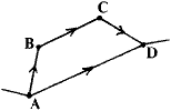
4) We now turn to the second, more useful, replacement theorem. Here we have two sections linking the same two vertex stations.
ie:  Note both sections are R->S.
| At R write | (7) | |
| At S write | (8) |
![]() 'e and
'e and
![]() ''e mean sum over
other sections attached to R and S respectively.
''e mean sum over
other sections attached to R and S respectively.
| We consider | [xS - xR -
|
| = [ n2 (xS - xR) - n2
| |
| = [ (n1 + n2) (xS - xR) -
n1
| |
| = [xS - xR - (n1
| |
| = [ xS - xR -
|
where we have put n = n1 n2 / (n1 + n2) ie. 1/n = 1/n1 + 1/n2
and ![]() =
(n1
=
(n1
![]() 2 -
n2
2 -
n2
![]() 1)
ie.
1)
ie. ![]() /n =
/n =
![]() 1 /
n1 +
1 /
n1 +
![]() 2 /
n2
2 /
n2
Put these results back into (7) and (8):
![]() 'e
- [xS - xR -
'e
- [xS - xR -
![]() ] / n = 0
] / n = 0
![]() ''e
+ [xS - xR -
''e
+ [xS - xR -
![]() ] / n = 0
] / n = 0
This shows we can replace  by
by 
Where 1/n = 1/n1 + 1/n2 and
![]() /n =
/n =
![]() 1 /
n1 +
1 /
n1 +
![]() 2 /
n2
2 /
n2
We now do another example to illustrate the utility of these replacement theorems.
Suppose we had to solve:
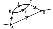 We have the following
data
| From | To | n | ||
|---|---|---|---|---|
| A | B | 3.45 | 5 | |
| B | C | 12.71 | 5 | [Route 1] |
| B | C | 12.29 | 7 | [Route 2] |
| C | D | 13.00 | 6 | |
| D | C | 28.37 | 18 |
Part 4) tells us we can replace the two routes from B to C by one with
![]() , n where:
, n where:
1/n = 1/5 + 1/7 or n = 2.92
and ![]() /n =
12.71/5 + 12.29/7 or
/n =
12.71/5 + 12.29/7 or
![]() = 12.54m
= 12.54m
So now we have
 B->C :
 ![]() =
12.54m, n = 2.92
=
12.54m, n = 2.92
Applying part 3) to the three sections A->B, B->C, C->D,
we have a second route from A to D with
![]() , n given by:
, n given by:
![]() = 3.45 + 12.54
+ 13.00 = 28.99m
= 3.45 + 12.54
+ 13.00 = 28.99m
n = 5 + 2.92 + 6 = 13.92
Hence we get
 where
where
![]() 4 =
28.99m, n4 = 13.92 from above
4 =
28.99m, n4 = 13.92 from above
![]() 3 =
28.37m , n3 = 18 from the table of data
3 =
28.37m , n3 = 18 from the table of data
We use part 4) again to get a single equivalent section from A to D with
![]() , n such that:
, n such that:
 1/n = 1/18 + 1/13.92 or n = 7.85
![]() /n =
28.37/18 + 28.99 / 13.92 or A = 28.72m
/n =
28.37/18 + 28.99 / 13.92 or A = 28.72m
We have done all the replacement we can, and have in fact solved the problem. We can now go back and calculate the positions of B and C.
Let's take xA = 0.00m as the basis station.
Then xD = 28.72m from the last result obtained.
The error back along route 4 from A to D is EAD4 = 28.72 - 28.99 = -0.27m
and the fractional error is e = -0.27/13.92 = -0.0193m
[Note we use the fractional values for n exactly as we would the integer values.]
Hence xB = xA +
![]() AB +
nAB.e = 0.00 + 3.45 + 5 x -0.0193 = 3.35m
AB +
nAB.e = 0.00 + 3.45 + 5 x -0.0193 = 3.35m
Similarly xC = xB +
![]() BC +
nBC.e = 3.35 + 12.54 +2.92 x -0.0193 = 15.83m
BC +
nBC.e = 3.35 + 12.54 +2.92 x -0.0193 = 15.83m
In summary
| xA = 0.00m | xC = 15.83m |
| xB = 3.35m | xD = 28.72m |
We can now calculate the errors along the various sections. We get:
| From | To | n | xTo - xFrom/m | E/m | e/m | |
|---|---|---|---|---|---|---|
| A | B | 3.45 | 5 | 3.35 | -0.10 | -0.0193 |
| B | C | 12.71 | 5 | 12.48 | -0.23 | -0.0462 |
| B | C | 12.29 | 7 | 12.48 | 0.19 | -0.0270 |
| C | D | 13.00 | 6 | 12.88 | -0.12 | -0.0193 |
| A | C | 28.37 | 18 | 28.72 | 0.35 | 0.0193 |
We are now back on familiar ground and could go on to distribute the errors back along the various sections, but since we already know how to do this, we stop here.
The replacement theorems mean that we can easily solve networks like these:
 or
or

where we have the problem of what to substitute in place of the smaller loops in the larger loops; and also how to distribute the errors back across the smaller loops.
Networks like the ones below are not amenable to such attack, and we have to use the general method instead (the last is the network at the beginning used as an example throughout).
 or
or
